Physics-based models (3): battery models, what’s your flavour?

We learned in our previous blog post that physics-based battery models typically impose conservation of lithium and charge in both the electrode and the electrolyte, but we did not discuss specific models. The focus of this post is on three of the most popular models: the Doyle-Fuller-Newman (DFN), the Single Particle Model (SPM) and the Single Particle Model with electrolyte dynamics (SPMe). They are all based on the same set of assumptions, as SPM and SPMe can be considered to be simplified versions of the DFN.

These models are very cleverly designed to capture the main features of a battery, while being relatively simple. They are built using the conservation laws and constitutive relations we explained in our previous post, but the clever part is that they are homogenised and multiscale. Homogenised means that, instead of capturing the intricate geometry of the porous material, the model assumes both the electrode and the electrolyte are a slab of homogeneous material. Then, the transport properties are adjusted to account for the fact that the material is actually porous (i.e. ions cannot move in a straight line but instead need to follow the intricate geometry).

Multiscale means that the models resolve separately the transport of intercalated ions, which occur at particle level (~ 1 μm), from all the other processes, which occur at cell level (~ 100 μm). By also assuming a simple geometry, the model can be reduced to two spatial coordinates (one for the particle radius and one for the cell thickness) and that is why the DFN model is also known as the pseudo-2-dimensional (P2D) model.

Both the homogenisation and multiscale assumptions make the DFN relatively simple. The Single Particle Models (with and without electrolyte) go one step further and approximates all the particles within an electrode by an averaged particle. Further simplifications can be made based on this assumption, which lead to a much simpler model in which we only need to solve equations for the concentration in the averaged particle of each electrode. If electrolyte dynamics are included (i.e. SPMe), one can also solve an equation for the concentration in the electrolyte, which does not add much complexity and significantly improves the accuracy of the model.

Figure 1: Comparison of SPM, SPMe and DFN for a 1C discharge. The code is available in this notebook.

PyBaMM allows to easily compare these models and observe the differences. In Figure 1, we show the comparison of the models for a 1C discharge. In terms of voltage, which is often the main variable we want to model, we observe a very good agreement between DFN and SPMe and some discrepancy between these two and the SPM (by SPM we mean with no electrolyte dynamics). Comparing other variables, like electrolyte concentration, we observe small discrepancies between DFN and SPMe, with a much more significant discrepancy of the SPM. As the name suggests, the SPMe is still a single particle model, so it does not capture concentration variations across the electrode thickness, but the discrepancy is quite small anyway.

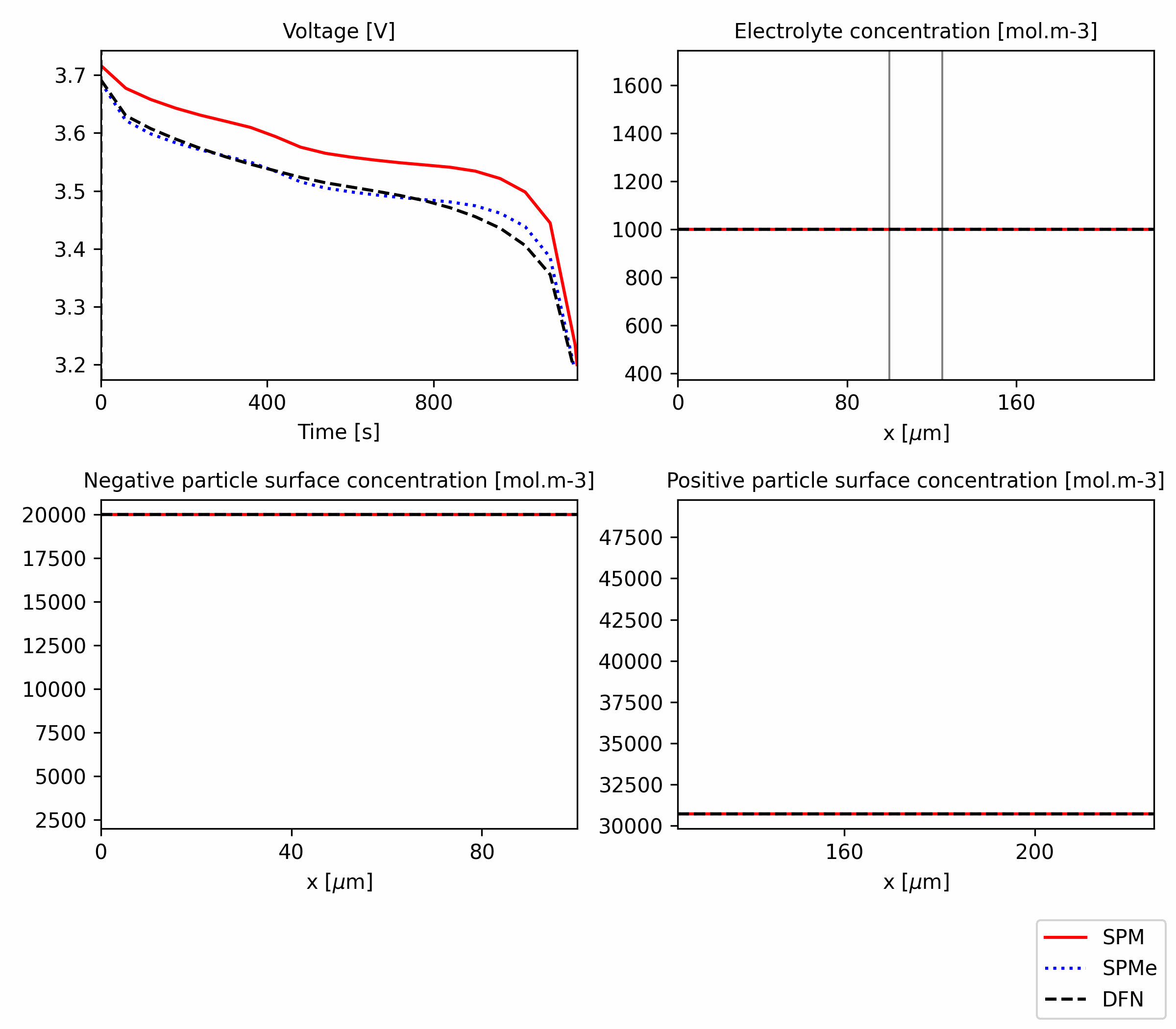
Figure 2: Comparison of SPM, SPMe and DFN for a 3C discharge. The code is available in this notebook.

The agreement of SPM and SPMe with DFN gets worse as the current increases. We can repeat the simulation but now for a 3C discharge to see the differences better. As shown in Figure 2, we observe that the agreement between DFN and SPMe is a bit worse, but it is still much better than the agreement between both and SPM. To understand why, we can check the voltage components.

Figure 3: Breakdown of the voltage components for SPM, SPMe and DFN. The code is available in this notebook.

The plots in Figure 3 show, for each model, the contribution of various phenomena to the final voltage curve (black dashed). We can observe that the main cause for the discrepancy between SPM and SPMe/DFN is that the former does not include the electrolyte overpotentials (concentration and Ohmic). It does not include the Ohmic electrode overpotential, but its contribution is quite small even for DFN and SPMe.

So far we have focused on the accuracy of the models, but not on the computational cost. PyBaMM automatically logs the solving time for the models. The actual times will depend on the specific machine, but we observe that SPM and SPMe have fairly similar solving times, which are two orders of magnitude smaller of that of the DFN model. Thus, solving the electrolyte equation in SPMe is a small price to pay given the significant increase in accuracy observed, making the SPMe a very good trade-off between computational cost and accuracy.

In our next blog post, we will discuss what are the main challenges of physics-based modelling and how Ionworks can help you overcome them.